Unit of Observation and S2 Cell Geometry
Yulia Zamriy
Overcoming data integration challenges using S2 cells.

Image credit: s2geometry.io
The Challenge of Combining the Data
The first challenge of the project was getting the data. Each data source came in a different geographic format:
- Weather: we obtained data for each weather station in California, with every weather station having specific coordinates (latitude and longitude).
- Fuel moisture: similar to weather data, we had a list of fuel moisture stations with their coordinates.
- Satellite imagery: each pixel of each satellite image came with meta data containing coordinates of a pixel centroid.
- Transmission lines: this data was available in a shapefile format where each transmission line was defined as a linestring object (a set of closely located points).
- Wildfire data: we downloaded a geodatabase file that contained wildfire perimeters since the 1800s.
Given all of the above, we faced our second challenge: how do we combine these datasets for our analysis? What is our common unit of observation?
How S2 Cells Fit Our Problem
After some research, we decided to use the S2 Cell Geometry methodolgy developed by Google. Our project required only a small part of its functionality, and that’s what we are going to focus in this blog post.
S2 Cell locations are static. An S2 Cell maps uniquely to an area on the Earth– think of it like a rectangular polygon drawn on the surface. Based on the documentation, there are 31 levels, with each level being 1/4 of its parent’s size (30 is the smallest cell size, and 0 is the largest cell size). At level 0 six cells cover the Earth. The S2 Cell containing a given point has a unique S2 Cell ID. A single point will belong to each S2 Cell level from 0 to 30, but each of the 31 different S2 Cell levels will still have its own unique identifier.
If you are interested in trying it out yourself, we created a Jupyter Notebook with instructions on how to get started. Please note that the S2 Cell library was created in C++ (see the GitHub repo for the source code), but there are wrapper libraries in Python as well. We used s2_py). It might take some time to set it up, but it’s feasible as we were able to run in on Linux (the easiest), Mac and Windows (via Docker).
The idea was to use an S2 Cell as our unit of observation: we would convert each data source into S2 Cells and merge them by S2 Cell IDs. But before merging the data, we had to create a baseline dataset - a universe of all S2 Cells covering California. And to do that we had to choose cell size. What size do we choose?
Selecting S2 Cell size
At first we wanted to choose a relatively small size (for example, level 13 or around 314 acres per cell) as it would allow us to have very granular data. However, this approach had two issues:
- The dataset was getting too large. There would be 390,415 S2 Cells of level 13 covering California. Then we would need to use each cell 1,096 times as we settled on using only 3 years of data for modeling (using more years would create even larger dataset size issues).
- Most of the data was not available at that level. For example, there are 4,778 weather stations in California. Hence, we would need to populate weather data in cells without weather stations by replicating weather from the nearest station in another cell.
As we kept increasing the cell size, it became clear that splitting California into the same size cells might not be an optimal solution. For example, deserts in the southeast had very few wildfires, while Northern California experienced many wildfires of various sizes.
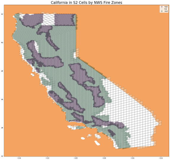
After much deliberation and weighing different options, we decided to split California into S2 Cells of 3 different sizes based on the historical occurence of wildfires. We downloaded fire zone perimeters from the National Weather Service and calculated the number of wildfires per zone. Then we split all California fire zones into 3 groups:
- Zones with low occurence of wild fires were split into 607 S2 Cells of level 9 (80,000 acres per cell)
- Zones with medium occurence of wild fires were split into 3,490 S2 Cells of level 10 (20,000 acres per cell)
- Zones with high occurence of wild fires were split into 6,546 S2 Cells of level 11 (5,000 acres per cell)
In total, California consisted of 10,643 S2 Cells. Hence, our final modeling dataset would consist of 11,664,728 observations (10,643 cells by 1,096 days).
Creating Our Final Dataset
To create our final dataset, we had to combine all the data sources. There are separate blog posts about each data source, but here’s a brief overview of how we converted each data source into S2 Cells:
- Weather and Fuel Moisure: find
S2 Cell IDsbased on coordinates of stations. For the cells without any stations, calculate distance from their centroids to each station, and assign weather/fuel moisture data from the nearest station. - Satellite imagery: using coordinates of each pixel’s centroid, find an
S2 Cellscontaining it. If anS2 Cellcontains multiple pixels, aggregate them. - Transmission lines: convert
LineStringobjects from Shapefiles intoS2 Polylineobjects. Then find allS2 Cellscovering thesePolylines. - Wildfire perimeters: convert
Polygonobjects from Shapefiles intoS2 Loopobjects. Then find allS2 Cellscovering theseLoops.
Each of the above had to be repeated 3 times for 3 selected cell sizes (9, 10, 11) before merging data into the baseline dataset by S2 Cell ID.